Algebra 2 Final Exam Review Plan
Preparation is key! Practice relentlessly, utilizing past exams and online resources like Khan Academy. Don’t just memorize; understand the concepts thoroughly.
Focus on identifying weaknesses through practice tests, then actively seek explanations and additional problems. Repeat this cycle until mastery is achieved.
Remember, consistent effort and a proactive approach to learning will significantly improve your performance and reduce exam-related stress.
I. Polynomial Functions
Mastering polynomial functions is foundational. Begin by confidently classifying polynomials based on degree and number of terms – crucial for understanding their behavior. Next, become proficient in polynomial operations: addition, subtraction, and multiplication. Practice combining like terms and distributing effectively.
Don’t shy away from polynomial division! Both long division and the more efficient synthetic division are vital skills. Understand the remainder theorem and its applications. Review identifying the degree of a polynomial and its standard form.
Utilize resources like past Regents exams and online videos to solidify your understanding. Focus on problems that require you to apply these concepts in various contexts. Remember, consistent practice is the key to success in this section.
A. Classifying Polynomials
Understanding polynomial classification is paramount. Polynomials are defined by their degree – the highest exponent of the variable – and the number of terms. A monomial has one term, a binomial has two, and a trinomial has three. Polynomials with more than three terms are simply referred to as polynomials.
Pay close attention to the degree of a polynomial; this dictates its end behavior. Linear polynomials have a degree of 1, quadratic polynomials a degree of 2, and cubic polynomials a degree of 3. Recognizing these forms is essential.
Practice identifying polynomials in standard form and determining their degree. Utilize online resources and practice problems to reinforce these concepts. Mastering this foundational skill will greatly aid in tackling more complex polynomial problems.
B. Polynomial Operations (Addition, Subtraction, Multiplication)
Proficiency in polynomial operations is crucial. Addition and subtraction involve combining like terms – terms with the same variable and exponent; Remember to distribute the negative sign during subtraction to avoid errors. Careful attention to signs is vital for accuracy.
Polynomial multiplication utilizes the distributive property. Multiply each term in the first polynomial by each term in the second polynomial, then combine like terms. This can be visualized using the FOIL method for binomials (First, Outer, Inner, Last).
Practice these operations extensively with various polynomial expressions. Online resources and practice problems will solidify your understanding. Mastering these skills forms the basis for more advanced polynomial manipulations.
C. Polynomial Division (Long Division & Synthetic Division)
Polynomial division encompasses two primary methods: long division and synthetic division. Long division mirrors traditional arithmetic long division, but with variables. It’s a versatile method applicable to any polynomial division problem, though it can be lengthy.
Synthetic division is a streamlined technique specifically for dividing a polynomial by a linear factor (of the form x – a). It’s faster and more efficient than long division, but requires careful setup and understanding of the process.
Practice both methods to become proficient. Pay close attention to placeholders for missing terms in the dividend. Understanding remainders and their significance is also essential. Utilize online tutorials and practice problems to reinforce these skills.
II. Quadratic Functions
Quadratic functions are fundamental in Algebra 2, appearing in numerous applications. Mastering them requires understanding different forms: standard (f(x) = ax² + bx + c), vertex (f(x) = a(x – h)² + k), and intercept (f(x) = a(x – r₁)(x – r₂)). Each form reveals key features.
The vertex form directly displays the vertex (h, k), crucial for finding maximum or minimum values. The standard form aids in identifying the y-intercept. Solving quadratic equations—factoring, using the quadratic formula, or completing the square—is vital.
Practice converting between forms and applying these techniques to real-world problems. Focus on interpreting the discriminant (b² ⎼ 4ac) to determine the nature of the roots.
A. Standard Form, Vertex Form, and Intercept Form
Understanding the three forms of a quadratic function is paramount. Standard form (f(x) = ax² + bx + c) is the most common, easily revealing the y-intercept at ‘c’. Vertex form (f(x) = a(x – h)² + k) immediately identifies the vertex at the point (h, k), representing either a maximum or minimum.
Intercept form (f(x) = a(x – r₁)(x – r₂)) showcases the x-intercepts, or roots, of the quadratic at r₁ and r₂. Converting between these forms is a crucial skill.
Practice completing the square to transform standard form into vertex form, and factoring to achieve intercept form. Recognizing the advantages of each form for specific problem-solving scenarios is key to success.
B. Finding the Vertex and Axis of Symmetry
The vertex represents the maximum or minimum point of a parabola. You can locate it using the formula x = -b / 2a, derived from the standard form (ax² + bx + c). Substitute this x-value back into the original equation to find the corresponding y-value, completing the vertex coordinates (x, y).
Alternatively, if the equation is already in vertex form, f(x) = a(x – h)² + k, the vertex is directly visible as (h, k). The axis of symmetry is a vertical line passing through the vertex, defined by the equation x = h.
Understanding this symmetry is vital; points equidistant from the axis of symmetry have the same y-value. Mastering these techniques allows for quick and accurate analysis of quadratic functions.
C. Solving Quadratic Equations (Factoring, Quadratic Formula, Completing the Square)
Mastering quadratic equation solutions is crucial. Factoring is quickest when applicable, involving finding two binomials that multiply to equal the quadratic expression. However, it doesn’t always work!
The quadratic formula, x = [-b ± √(b² ⎼ 4ac)] / 2a, always provides solutions, even with complex roots. Completing the square transforms the equation into vertex form, enabling solution finding by taking the square root of both sides.
Practice each method extensively. Recognize when factoring is efficient, and when the formula or completing the square is necessary. Understanding the discriminant (b² ー 4ac) reveals the nature of the roots – real, distinct, or complex.

III. Exponential and Logarithmic Functions
Exponential functions demonstrate rapid growth or decay, modeled by y = a * bx. Understanding ‘a’ (initial value) and ‘b’ (growth/decay factor) is paramount. Logarithmic functions are their inverses, used to solve for exponents.
Key properties of logarithms include product, quotient, and power rules – essential for simplifying expressions and solving equations. Remember that logb(x) = y means by = x.
Practice converting between exponential and logarithmic forms. Solving equations often involves isolating the exponential or logarithmic term, then applying inverse operations. Be mindful of domain restrictions for logarithms (argument must be positive).
A. Exponential Growth and Decay
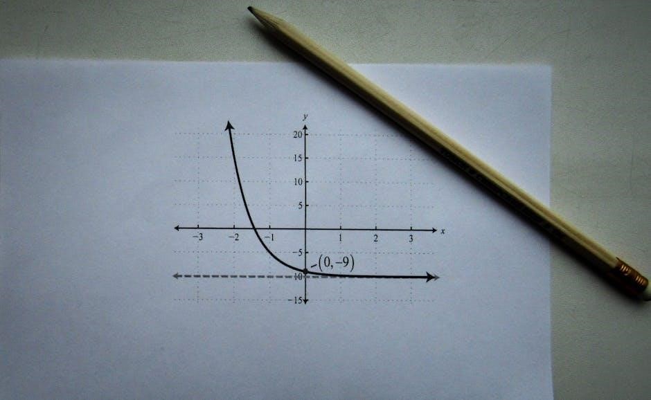
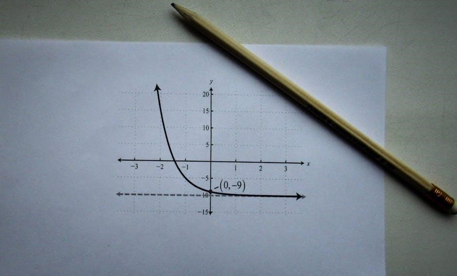
Exponential growth occurs when the base ‘b’ is greater than 1, resulting in an increasing function. Real-world examples include population growth and compound interest. Exponential decay, where ‘b’ is between 0 and 1, models phenomena like radioactive decay and depreciation.
The general formula is y = a(1 ± r)t, where ‘r’ represents the rate of growth or decay (expressed as a decimal). Positive ‘r’ signifies growth, while negative ‘r’ indicates decay. ‘t’ represents time.
Master identifying growth versus decay from an equation and interpreting the rate. Practice applying these concepts to word problems, carefully noting the initial value, rate, and time period. Understanding half-life is crucial for decay problems.
B. Properties of Logarithms
Logarithms are the inverse of exponential functions, and understanding their properties is vital for solving equations. Key properties include the product rule (logb(mn) = logb(m) + logb(n)), the quotient rule (logb(m/n) = logb(m) ⎼ logb(n)), and the power rule (logb(mp) = p*logb(m)).
The change-of-base formula (loga(x) = logb(x) / logb(a)) allows converting logarithms to a common base, often base 10 or ‘e’. Remember that logb(1) = 0 and logb(b) = 1.
Practice applying these properties to condense or expand logarithmic expressions, and to simplify complex equations. Mastery of these rules is essential for efficiently solving exponential and logarithmic equations.
C. Solving Exponential and Logarithmic Equations
Solving exponential equations often involves isolating the exponential term and then applying logarithms to both sides. Remember to choose a logarithm base that corresponds to the base of the exponential function, or utilize the change-of-base formula. Be vigilant for extraneous solutions, as logarithms are not defined for non-positive numbers.
For logarithmic equations, aim to condense the logarithmic terms into a single logarithm using the properties discussed previously. Then, convert the equation to exponential form to solve for the variable. Again, always check your solutions to ensure they don’t result in the logarithm of a non-positive number.
Practice is crucial for recognizing patterns and applying the correct techniques efficiently.
IV. Rational Expressions and Equations
Simplifying rational expressions requires factoring both the numerator and denominator, then canceling any common factors. Remember to identify values of the variable that would make the denominator zero – these are restrictions on the variable’s domain and must be noted.
Operations with rational expressions (addition, subtraction, multiplication, and division) follow similar rules to operations with fractions. Finding a common denominator is essential for addition and subtraction. Multiplication involves multiplying numerators and denominators, while division involves multiplying by the reciprocal.

Solving rational equations involves finding a common denominator, eliminating the fractions, and solving the resulting polynomial equation. Always check for extraneous solutions by substituting back into the original equation.
A. Simplifying Rational Expressions

Simplification is paramount! Begin by completely factoring both the numerator and the denominator of the rational expression. Look for common factors – these are the keys to reducing the expression to its simplest form. Remember, factoring can involve various techniques like greatest common factor, difference of squares, or trinomial factoring.
Crucially, identify any values of the variable that would result in a zero denominator in the original expression. These values represent restrictions on the variable and must be explicitly stated, as they are not part of the domain.
Finally, cancel out the common factors. Ensure the simplified expression is fully reduced, with no remaining common factors between the numerator and denominator.

B. Operations with Rational Expressions (Addition, Subtraction, Multiplication, Division)
Mastering these operations is vital! For addition and subtraction, find a common denominator – often the least common multiple (LCM) of the denominators. Rewrite each expression with this common denominator, then combine the numerators.
Multiplication is straightforward: multiply the numerators together and the denominators together, then simplify the resulting expression. Division requires inverting the second fraction (the divisor) and then multiplying, again simplifying afterwards.
Remember to always factor before performing any operation, as this can reveal opportunities for cancellation and simplification. Always state any restrictions on the variable derived from the original denominators.
C. Solving Rational Equations
Solving rational equations requires a careful approach! Begin by identifying the least common denominator (LCD) of all fractions within the equation. Multiply every term on both sides of the equation by the LCD. This crucial step eliminates the fractions, transforming the equation into a more manageable polynomial form.
Next, solve the resulting polynomial equation using familiar techniques like factoring or the quadratic formula. Crucially, always check your solutions by substituting them back into the original rational equation.
Beware of extraneous solutions! These are values that satisfy the polynomial equation but render the original rational equation undefined (due to division by zero). Discard any extraneous solutions. Always note domain restrictions!
V. Radical Functions and Equations
Mastering radical functions and equations demands precision! Begin by isolating the radical expression on one side of the equation. Then, raise both sides of the equation to a power that will eliminate the radical – squaring is common for square roots, cubing for cube roots, and so on.
However, this step can introduce extraneous solutions, so diligent verification is paramount. Substitute each potential solution back into the original radical equation to confirm its validity. Any solution that doesn’t satisfy the original equation must be discarded.
Simplifying radical expressions involves factoring out perfect square (or cube, etc.) factors from under the radical sign. Remember to always check for domain restrictions when dealing with radicals, as negative values under even roots are undefined.
A. Simplifying Radical Expressions
Simplifying radicals is foundational! The core principle involves identifying and extracting perfect square (or cube, etc.) factors from beneath the radical symbol. For instance, √12 can be simplified to 2√3, as 12 contains the perfect square factor of 4.
Remember to factor completely – don’t stop at the first perfect factor you find. Also, ensure the radicand (the expression under the radical) has no remaining factors that can be simplified. Pay close attention to coefficients; they are multiplied after simplification.
Rationalizing the denominator is often required when the denominator contains a radical. Multiply both numerator and denominator by the conjugate of the denominator to eliminate the radical from the bottom. This ensures a simplified and standard form.
B. Solving Radical Equations
Isolate the radical first! This is the crucial initial step. Manipulate the equation algebraically to get the radical expression by itself on one side of the equation. Then, raise both sides to the appropriate power to eliminate the radical – squaring both sides is common for square roots.
Be vigilant for extraneous solutions! This is paramount. After solving, always substitute your solutions back into the original equation to verify their validity. Radical equations can sometimes produce solutions that don’t actually satisfy the original equation.

Handle multiple radicals carefully. If multiple radicals are present, isolate one, eliminate it, and then repeat the process for any remaining radicals. Remember to check all potential solutions for extraneous values.
VI; Complex Numbers
Recall the definition: Complex numbers are expressed in the form a + bi, where ‘a’ is the real part and ‘b’ is the imaginary part, and ‘i’ represents the square root of -1. Mastering operations with these numbers is vital.
Addition and subtraction involve combining like terms – real with real, and imaginary with imaginary. Multiplication utilizes the distributive property, remembering that i2 = -1. Division requires multiplying both numerator and denominator by the complex conjugate of the denominator.
Powers of ‘i’ follow a pattern: i1 = i, i2 = -1, i3 = -i, and i4 = 1. This cycle repeats, simplifying higher powers of ‘i’ significantly. Practice recognizing this pattern!
A. Operations with Complex Numbers (Addition, Subtraction, Multiplication, Division)
Addition and subtraction of complex numbers are straightforward: combine the real parts and the imaginary parts separately. For example, (2 + 3i) + (1 ⎼ i) = (2+1) + (3-1)i = 3 + 2i.
Multiplication requires applying the distributive property (FOIL method) and remembering that i2 = -1. So, (a + bi)(c + di) = ac + adi + bci + bdi2 = (ac ー bd) + (ad + bc)i.
Division is more involved. Multiply both the numerator and denominator by the complex conjugate of the denominator. This eliminates the imaginary part from the denominator. The conjugate of (c + di) is (c ⎼ di). Practice these steps diligently!
B. Powers of i
Understanding the cyclical nature of i’s powers is crucial. Remember that i is defined as the square root of -1. Therefore: i1 = i, i2 = -1, i3 = -i, and i4 = 1.
After i4, the pattern repeats! This means any higher power of i can be simplified by finding the remainder when the exponent is divided by 4. For instance, i11 is the same as i3 (since 11 divided by 4 has a remainder of 3), which equals -i.
Mastering this pattern will save you significant time on the final exam. Practice simplifying various powers of i to solidify your understanding and avoid common errors.
VII. Trigonometry
Trigonometry in Algebra 2 heavily emphasizes the unit circle. Familiarize yourself with its key angles (0, 30, 45, 60, 90 degrees and their radian equivalents) and the corresponding (x, y) coordinates. These coordinates directly relate to cosine and sine values, respectively.
Understand how to determine all six trigonometric functions (sine, cosine, tangent, cosecant, secant, cotangent) from the unit circle. Practice identifying reference angles and understanding how signs change in different quadrants.
Be prepared to sketch graphs of trigonometric functions and identify their amplitude, period, and phase shift. Knowing these concepts will be vital for solving related problems on the final exam.
A. Unit Circle
The unit circle is foundational to understanding trigonometric functions. It’s a circle with a radius of one, centered at the origin of a coordinate plane. Mastering it is crucial for success on your Algebra 2 final!
Focus on memorizing the coordinates of key angles: 0, 30, 45, 60, and 90 degrees (and their radian equivalents). These coordinates directly correspond to cosine and sine values – the x and y coordinates, respectively.
Practice identifying reference angles, which are acute angles formed between the terminal side of an angle and the x-axis. Understanding how trigonometric function signs change in each quadrant is also essential. Utilize online resources and practice problems to solidify your understanding.

B. Trigonometric Functions and their Graphs
Understanding the graphs of sine, cosine, and tangent functions is vital. Each function possesses unique characteristics – amplitude, period, phase shift, and vertical shift – that dictate their shape and position on the coordinate plane.
The amplitude determines the height of the wave, while the period defines the length of one complete cycle. Phase shifts move the graph horizontally, and vertical shifts move it vertically. Practice identifying these features from the equation of each function.
Recognize the reciprocal relationships between trigonometric functions (e.g., secant is the reciprocal of cosine). Utilize graphing calculators or online tools to visualize these functions and confirm your understanding. Consistent practice is key to mastering these concepts!